Gaussian processes
This week I discuss a lecture by David MacKay on “Gaussian Process Basics”. Unfortunately, the video on that website requires Flash support, which is obsolete and I am not going to install it. Luckily, someone seems to have uploaded a recording to YouTube. To understand this post, you need to have a basic understanding of linear algebra and be somewhat familiar with probability theory.
In my own words
A Gaussian process (GP) is a mathematical tool that, just like neural networks (NNs), can be used to learn a probability distribution from data, i.e. to do regression, classification, and inference.
GPs are a generalization of multivariate Gaussian (a.k.a. Normal) distributions. The (multivariate) Gaussian distribution is fully characterized by a mean vector \pmb{\mu} and a positive definite, symmetric covariance matrix \mathbf{\Sigma}. Its probability density function is
P(\mathbf{y}|\pmb{\mu}, \mathbf{\Sigma}) = \frac{1}{Z}\,\exp\biggl(-\frac{1}{2}\,(\mathbf{y} - \pmb{\mu})^{\rm{T}}\cdot\mathbf{\Sigma}^{-1}\cdot(\mathbf{y} - \pmb{\mu})\biggr)\;,where Z is a normalization factor that only depends on \mathbf{\Sigma}. Notice, that the right hand side contains the inverse of \mathbf{\Sigma}.
MacKay explains very clearly how these “boring old Gaussian distributions” can be used for things like inference. First, we consider the two-dimensional case, where the above probability density may be written as
P(y_1, y_2|\mathbf{\Sigma}) = \frac{1}{Z}\,\exp\biggl(-\frac{1}{2}\,\left(\begin{array}{cc} y_1 & y_2 \end{array}\right)\cdot\mathbf{\Sigma}^{-1}\cdot\left(\begin{array}{c} y_1 \\ y_2\end{array}\right)\biggr)\;.Here, we assume that \pmb{\mu} = (0, 0), for simplicity.
A sample from that distribution is sometimes displayed as a dot in a contour plot of the probability density function (see left panel of Figure 1, below). But we can also represent it by displaying the two coordinates of the sample point separately, as in the right panel of Figure 1.
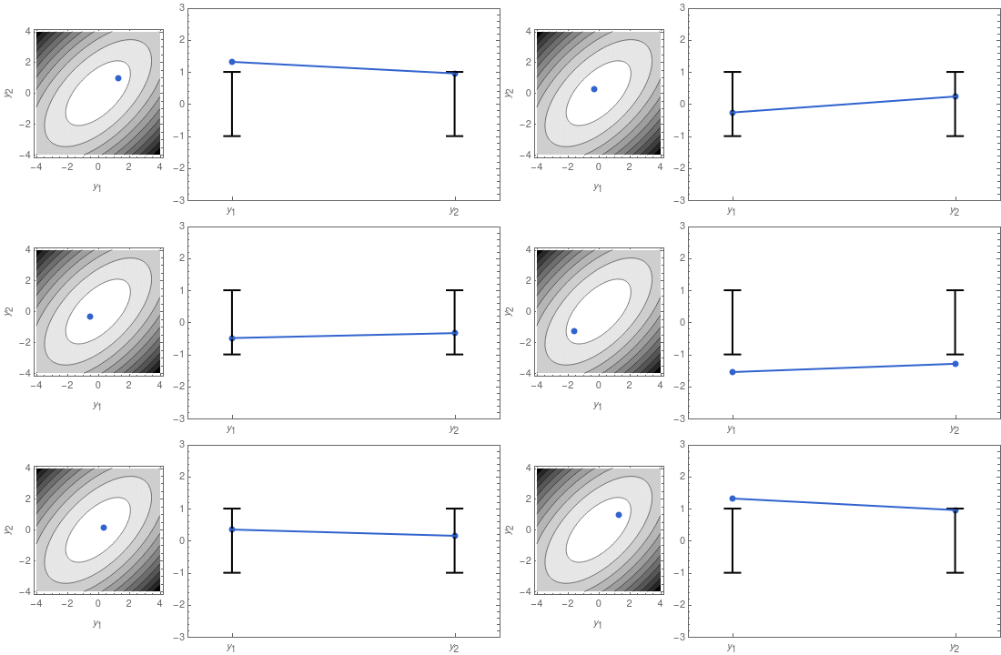
On the right panel of Figure 1 I also display the confidence intervals, given by the mean \mu_i = 0, and the standard deviations \sigma_1 and \sigma_2. The latter are the square roots of the diagonal elements of \mathbf{\Sigma}:
\mathbf{\Sigma} = \left(\begin{array}{cc}\sigma_1^2 & \rho\,\sigma_1\,\sigma_2 \\ \rho\,\sigma_1\,\sigma_2 & \sigma_2^2\end{array}\right)\;.Note, that in the right panel of Figure 1 there is some correlation between the height of the left dot, and the height of the right dot. The strength of that correlation is controlled by the factor \rho in the equation above. If \rho = 0, then there is no correlation, the left and right point’s positions would be unrelated, and the contour plot would show perfect circles.
What if we take a “measurement”, and the y_1 coordinate is known? What do we learn about the distribution of y_2? In other words, we would like to know the probability to get y_2, given y_1, which is
P(y_2 | y_1, \mathbf{\Sigma}) = \frac{P(y_1, y_2|\mathbf{\Sigma})}{P(y_1|\mathbf{\Sigma})}\;.But this is again a Gaussian distribution! Specifically, in this 2-dimensional case we find
P(y_2 | y_1, \mathbf{\Sigma}) \propto \exp\biggl(-\frac{1}{2}\,(y_2 - \mu_{y_2})^2\,\Sigma_{y_2}\biggr)\;,where
\mu_{y_2} = \frac{\rho\,\sigma_1\,\sigma_2}{\sigma_1^2}\,y_1 \;\;\;,\;\;\;\Sigma_{y_2} = \sigma_2^2\,(1 - \rho^2)\;.In Figure 2 I recreate Figure 1 with y_1 fixed, using the formulas above.
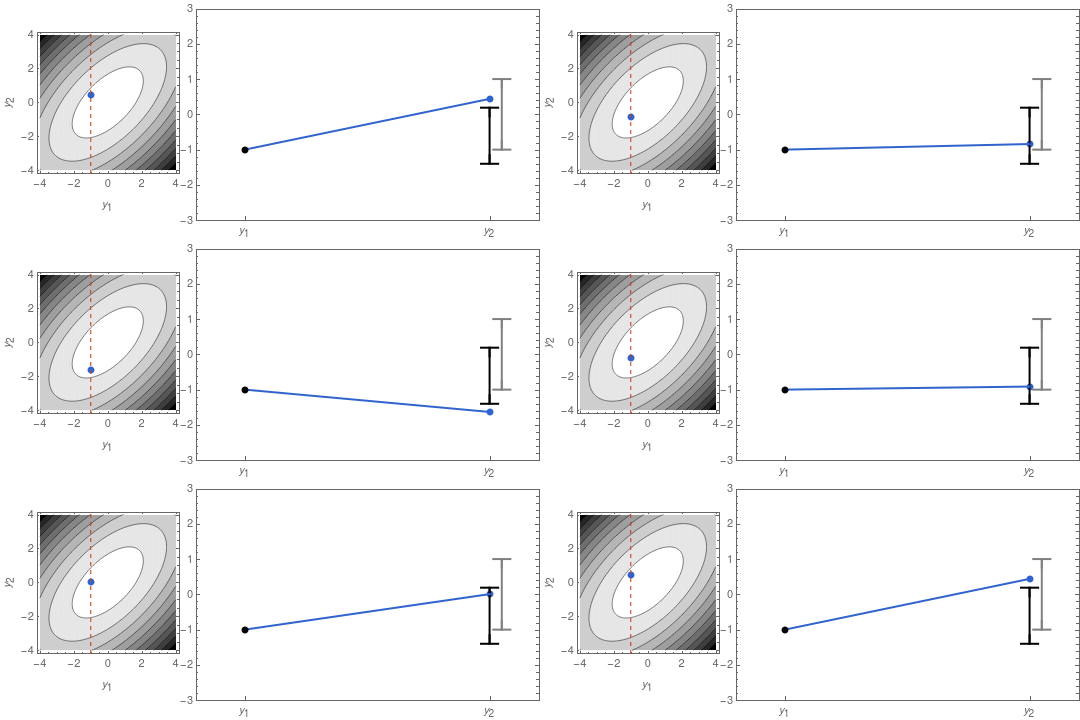
The advantage of the representation depicted in the right panels of Figures 1 and 2 is, that it can be easily generalized to higher dimensions. Can you see how this might lead us to a method for function approximation?
The idea is, that we can send the number of dimensions to infinity. So we have an infinite collection of correlated Gaussian random variables, each representing the function value at one input. This can be conceived as a distribution over functions, and the graphical representation in the right panels of Figure 1 and 2 is related to the possible graphs of these functions.
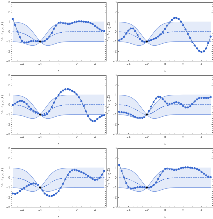
To make this more concrete, here are some samples from a 40-dimensional Gaussian distribution:
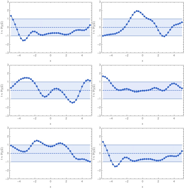
If we have infinitely many dimensions, then the Gaussian distribution has to be described in terms of a mean function, and a covariance function. We can then sample from the distribution in a finite dimensional subspace because of the property of a multivariate Gaussian that also defines a GP:
A Gaussian process is a collection of random variables, any finite number of which have a joint Gaussian distribution .
In other words, if we want to sample one function from a GP, we may begin by sampling one value y_1. Having drawn that sample, the GP is now conditioned on that sample, so that the value of y_2 will depend on it through the covariance function and y_1 in a similar way as we have seen in the two-dimensional example.

For the example shown above, I chose the common exponential covariance function
k(x_1, x_2) = \sigma^2\,\exp\bigl(-(x_1 - x_2)^2 / (2\,l^2)\bigr)The covariance matrix \mathbf{\Sigma} can now be generated by evaluating k(x_1, x_2) at all pairs of the x-coordinates that we are interested in.
In the exponential covariance function above, the correlation length l determines how far the effect of fixing y_1 should reach. If l is sent to 0, then there is no correlation between any two points of the function, and we will not obtain a smooth graph. For increasingly large l, the sampled functions will tend to become increasingly smooth.
The \sigma parameter is the signal variance, which determines the variation of function values from their mean. It is also common to add a noise variance \delta_{ij}\,\sigma_{\nu}^2 to the kernel k(x_1, x_2), where \sigma_{\nu} describes how much noise is expected to be present in the data.
MacKay also considers other covariance functions, and discusses why we write the distribution in terms of \mathbf{\Sigma} instead of \mathbf{\Sigma}^{-1}. Have a look at his lecture for those details.
Opinion, and what I have learned
Just like his book , MacKay’s lecture is exceptionally insightful. In particular, he provides several enlightening exercises (sometimes with solutions) in both his book and during his lecture. Therefore, I highly recommend both to anyone who is mathematically inclined.
Form this lecture, I have not only gained a rough understanding of what a GP is, but now it is also more clear to me what people mean by “non-parametric models” of which the GP is an example.
This is only an introduction to GPs, of course, and for more details, MacKay recommends the book by Rasmussen and Williams , as well as his own book . I, however, will not spend more time on GPs in the near future, and instead explore the newly invented framework of neural processes in my next Article of the Week.
