Conditional neural processes

This week’s article is “Conditional Neural Processes” by Garnelo et al. . To understand this post, you need to have a basic understanding of neural networks and Gaussian processes.

In my own words

A neural process (NP) is a novel framework for regression and classification tasks that combines the strengths of neural networks (NNs) and Gaussian processes (GPs) . In particular, similar to GPs, NPs learn distributions over functions and predict their uncertainty about the predicted function values. But in contrast to GPs, NPs scale linearly with the number of data points (GPs typically scale cubically ). A well-known special case of an NP is the generative query network (GQN) that has been invented to predict 3D scenes from unobserved viewpoints .

Neural processes should come in handy for several parts of my Rubik’s Cube project. Thus, I aim to build a Python package that lets the user implement NPs and all their variations with a minimal amount of code. As a first step, here I reproduce some of Garnelo et al.’s work on conditional neural processes (CNPs), which are the precursors of NPs.

If you just want to know what you can do with CNPs, feel free to skip ahead to the next section, but a little bit of mathematical background can’t hurt 🙂

Consider the following scenario. We want to predict the values \boldsymbol{y}^{(t)} = f(\boldsymbol{x}^{(t)}) of an (unknown) function f at a given set of target coordinates \boldsymbol{x}^{(t)}. We are provided with a set of context points {\boldsymbol{x}^{(c)}, \boldsymbol{y}^{(c)}} at which the function values are known, i.e. \boldsymbol{y}^{(c)} = f(\boldsymbol{x}^{(c)}). In addition, we can look at an arbitrarily large set of graphs of other functions that are members of the same class as f, i.e. they have been generated by the same stochastic process. A CNP solves this prediction problem by training on these other functions, thereby parametrizing the stochastic process with an NN.

Specifically, the CNP consists of three components: an encoder, an aggregator, and a decoder. The encoder h is applied to each context point (x_i^{(c)}, y_i^{(c)}) and yields a representation vector \boldsymbol{r}_i of that point. The aggregator is a commutative operation \oplus that takes all the representation vectors {\boldsymbol{r}_i} and combines them into a single representation vector \boldsymbol{r} = \boldsymbol{r}_1 \oplus \dots \oplus \boldsymbol{r}_n. In this work, the aggregator simply computes the mean. Finally, the decoder g takes a target coordinate x_i^{(t)} and the representation vector \boldsymbol{r}, and (for regression tasks) predicts the mean and variance for each function value that is to be estimated.

Here, both h and g are multi-layer perceptrons (MLPs) that learn to parametrize the stochastic process by minimizing the negative conditional log-probability to find \boldsymbol{y}^{(t)}, given the context points and \boldsymbol{x}^{(t)}.

Ok, now to applications. I reproduced two of the application examples that Garnelo et al. demonstrate. I plan to add more results and a generalization to NPs at a later stage. Please refer to my GitHub repository for updates.

As a first example, we generate functions from a GP with a squared-exponential kernel and train a CNP to predict these functions from a set of context points. After only 10^5 episodes of training, the CNP already performs quite well:

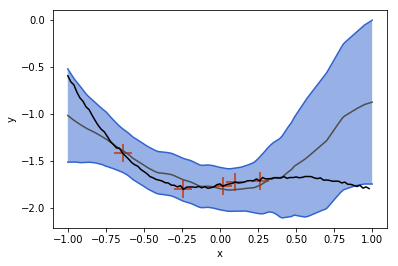
In the plot above, the gray line is the mean function that the CNP predicts, and the blue band is the predicted variance. For this example, the CNP is provided with the context points indicated by red crosses. as well as 100 target points on the interval [-1,1] that constitute the graph.

Notice that the CNP is less certain in regions far away from the given context points (see left panel around x \approx 0.75). When more points are given, the prediction improves and the uncertainty decreases.

In contrast to a GP, however, the CNP does not predict exactly the context points, even though they are given.

Of course, a GP with the same kernel as the GP that the ground truth function was sampled from performs better:

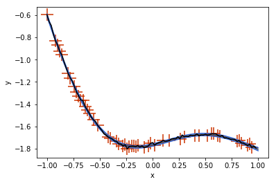
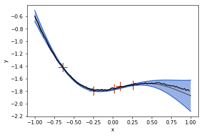
but this is kind of an unfair comparison, since the CNP had to “learn the kernel function” and we did not spend much time on training.

Now comes the really cool thing about CNPs. Since they scale linearly with the number of sample points, and since they can learn to parametrize any stochastic process, we can also conceive the set of all possible handwritten digit images as samples from a stochastic process and use a CNP to learn them.

After just 4.8\times10^5 training episodes, the same CNP that I used for 1-D regression above, has learned to predict the shapes of handwritten digits, given a few context pixels:

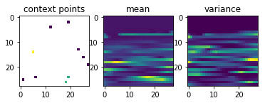
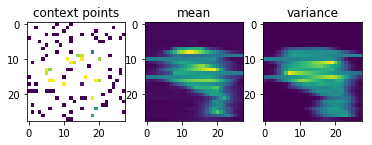
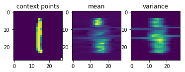
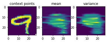
Garnelo et al.’s results look much nicer than mine, but my representation vector was only half the size of the one they used and they probably also spent more resources on training the CNP.

Opinion, and what I have learned

CNPs and their generalizations promise great potential, as they alleviate the curse of dimensionality of Gaussian processes and have already shown to be powerful tools in the domain of computer vision .

Garnelo et al. provide enough details about the implementation, so it was straightforward to reproduce their work. I only encountered one minor issue: When training the CNP, I sometimes find that it outputs NaN values. This problem disappears if we enforce a positive lower bound on the output variance.

Implementing CNPs was a good exercise for me to learn more about Tensorflow. Since the results are very rewarding and implementation is not too difficult, I recommend you try this yourself!

There are quite a few things that can be improved upon CNPs, which leads us to NPs and their extensions. But this is material for a later post.

References