Seven Scientists
In this post, I discuss one of my favorite problems from MacKay’s fantastic book on information theory . As the title suggests, the problem concerns seven scientists, and it illustrates the weakness of maximum likelihood estimation.
Maximum likelihood
The problem comes in two parts. In the first part, we use the maximum likelihood heuristic to solve the following problem:
N datapoints \{x_n\} are drawn from N distributions, all of which are Gaussian with mean \mu, but with different unknown standard deviations \sigma_n. What are the maximum likelihood parameters \mu, \{\sigma_n\}, given the data?
For example, seven scientists (A, B, C, D, E, F, G) with widely-differing experimental skills measure \mu. You expect some of them to do accurate work (i.e. to have small \sigma_n), and some of them to turn in wildly inaccurate answers (i.e. to have enormous \sigma_n). […] What is \mu and how reliable is each scientist?
MacKay, exercise 22.15.
In the book, the seven results by the seven scientists A to G are: -27.02, 3.57, 8.191, 9.898, 9.603, 9.945, and 10.056, respectively, as shown in this Figure:

To find the maximum likelihood values, we find the fixed point of the following rule:
\sigma_i \leftarrow \left|x_i - \frac{1}{N}\,\sum_{k = 1}^N \frac{x_k}{\sigma_k^2}\right|\;,resulting in \mu = 0.1.

The dashed red line in Figure 2 indicates the maximum likelihood estimate of \mu, and error bars indicate the estimated standard deviation of each scientist.
Bayesian approach
The second part of the problem assesses the same situation with the full power of Bayesian statistics:
Give a Bayesian solution to exercise 22.15, where seven scientists of
MacKay, exercise 24.3.
varying capabilities have measured \mu with personal noise levels \sigma_n, and we are interested in inferring \mu. Let the prior on each \sigma_n be a broad prior, for example a gamma distribution with parameters (s, c)= (10, 0.1). Find the posterior distribution of \mu. Plot it, and explore its properties for a variety of data sets such as the one given, and the data set \{x_n\} = \{13.01, 7.39\}.
So, we assume that the \sigma_n come from a gamma distribution, i.e.
P(\sigma) = \frac{1}{\Gamma(c)\,s}\,\biggl(\frac{\sigma}{s}\biggr)^{c - 1}\,\exp\biggl(-\frac{\sigma}{s}\biggr)\;,where \Gamma is the gamma function. Furthermore, if we’d know \mu and \sigma, then the probability to measure x is given by a Gaussian distribution
P(x|\mu, \sigma) = \frac{1}{\sqrt{2\,\pi}}\,\exp\biggl(-\frac{(x - \mu)^2}{2\,\sigma^2}\biggr)\;,and we want to know P(\mu | \{x_n\}).
Estimating noise levels
As a first step, we seek the nth scientist’s noise level P(\sigma_n | \mu, x_n), which is given by Bayes’ theorem as
P(\sigma_n | \mu, x_n) = \frac{P(x_n | \mu, \sigma_n)\,P(\sigma_n)}{P(x_n | \mu)}\;,where we’ve used that P(\sigma_n | \mu) = P(\sigma_n).
We already know the numerator of the right hand side. So we only need to find the normalizing constant P(x_n | \mu) by marginalizing P(x_n|\mu, \sigma_n) over \sigma_n, i.e. we integrate P(x|\mu, \sigma)\,P(\sigma) over \sigma from 0 to infinity:
P(x_n | \mu) = \int_0^\infty\;P(x_n | \mu, \sigma_n)\,P(\sigma_n)\,\rm{d}\sigma_n\;.We solve this integral analytically and find
\begin{aligned}P(x_n | \mu) =& \frac{1}{2\,\sqrt{\pi}\,s^2\,\Gamma(c)}\Biggl(\sqrt{2}\,\Gamma(c - 2)\,{}_0F_2\biggl(;\frac{3-c}{2}, \frac{4 - c}{2}; -\frac{(x_n - \mu)^2}{8\,s^2}\biggr) \\ &+ 2^{(1-c)/2}\,s^{2-c}\,|x_n - \mu|^{c-2}\,\Gamma\biggl(\frac{2 - c}{2}\biggr)\,{}_0F_2\biggl(;\frac{1}{2}, \frac{c}{2}; -\frac{(x_n - \mu)^2}{8\,s^2}\biggr) \\ &-\;\;\; 2^{-c/2}\,s^{1-c}\,|x_n - \mu|^{c-1}\,\Gamma\biggl(\frac{1-c}{2}\biggr)\,{}_0F_2\biggl(;\frac{3}{2}, \frac{c + 1}{2}; -\frac{(x_n - \mu)^2}{8\,s^2}\biggr)\Biggr)\;,\end{aligned}where {}_0F_2 is the generalized hypergeometric function.
We now have everything we need to plot P(\sigma_n | x_n, \mu). If we would assume that \mu = 10, then we’d find that we’re quite uncertain about the noise level of scientist A, but it is generally large, while we are very certain about the noise levels of scientists D, F and G, which should be small, as you can see in Figure 3.

If we instead assumed the \mu that we found with the maximum likelihood estimate, \mu = 0.1, then we’d be relatively sure that B’s noise level is lower than all other noise levels (see Figure 4), which is consistent with Figure 2.

The distribution of \mu
In the previous section we have found an expression for P(x_n | \mu). Since all measurements are independent from one another, the probability to find all the x_n is
P(\{x_n\} | \mu) = \prod_{n = 1}^N\,P(x_n | \mu)\;,where N = 7 is the number of scientists.
Now we use Bayes’ theorem again to find
P(\mu | \{x_n\}) = \frac{P(\{x_n\} | \mu)\;P(\mu)}{P(\{x_n\})} \propto P(\{x_n\} | \mu)\;.We don’t know anything about the prior P(\mu), but we could assume that it’s a uniform distribution between some large negative and positive values. In this case, P(\mu | \{x_n\}) is proportional to P(\{x_n\} | \mu), as indicated above.
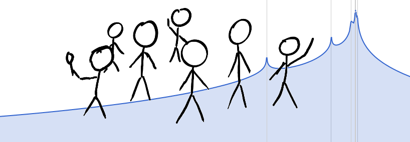
Inserting the given values for the parameters c and s, we can now plot P(\mu | \{x_n\}) in Figure 5 (vertical scales are not given, since we have not computed the normalization).

The graph in Figure 5 diverges to +\infty for every \mu = x_n. The probability density around these singularities accumulates when multiple data are close to one another, resulting in an increased probability to find \mu around \mu = 10.
Another dataset
MacKay also asks what happens if we had just two scientists, measuring \{x_n\} = \{13.01,7.39\}. As we would expect, the probability distribution over \mu is exactly symmetric:

This symmetry reflects the fact that with just two measurements, we cannot decide which scientist is the more accurate one, and therefore, we cannot know if 13.01 or 7.39 is closer to the true \mu.