Do all Snickers bars taste the same?
Last year, I noticed that Snickers bars seem to taste different in different countries, but I was not sure. So my partner Nellissa and I conducted a little experiment that involved a lot of chocolate and a little Bayesian statistics.
We wanted to establish whether Snickers bars from different countries taste different or not. To this end, we collected three Snickers bars, one from England (GB), one from Germany (DE), and one from Vietnam (VN). There are five plausible hypothesis:
- All Snickers bars taste the same: \mathcal{H}_{=}
- All Snickers bars taste different: \mathcal{H}_{\neq}
- The German and English bars are identical, but the Vietnamese is different: \mathcal{H}_{VN}
- The German and Vietnamese bars are identical, but the English is different: \mathcal{H}_{GB}
- The English and Vietnamese bars are identical, but the German is different: \mathcal{H}_{DE}
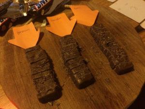
During the experiment we sliced the three bars into 12 slices each. Then we randomly paired slices and assessed whether they tasted the same or not. For example, one measurement may result in the observation \rm{DE} = \rm{GB} and another measurement may result in \rm{GB} \neq \rm{VN}. In addition, we also compare Snickers bars to themselves, so we might obtain \rm{VN} = \rm{VN}. We can perform a Bayesian update (explained below) on the above hypotheses after each measurement.
The measurement is subjective and may be affected by substantial noise. In particular, given two samples the experimenter may decide they taste different, even though they are equal, or vice versa. For simplicity, we assume a single failure rate \epsilon for all experiments. Given one sample pair, the probability that any experimenter misjudges the equality of the samples is \epsilon, thus \epsilon \in [0,1].
To make the five hypotheses that we have introduced above more explicit, we write down the outcome probabilities of an experiment (likelihoods), given that the hypothesis k is true and \epsilon is known.
For the all-equal hypothesis \mathcal{H}_{=} we have:
P(\rm{DE} = \rm{UK}\,|\,\mathcal{H}_{=}, \epsilon) = P(\rm{DE} = \rm{VN}\,|\,\mathcal{H}_{=}, \epsilon) = P(\rm{UK} = \rm{VN}\,|\,\mathcal{H}_{=}, \epsilon) = 1 - \epsilon\;, P(\rm{DE} \neq \rm{UK}\,|\,\mathcal{H}_{=}, \epsilon) = P(\rm{DE} \neq \rm{VN}\,|\,\mathcal{H}_{=}, \epsilon) = P(\rm{UK} \neq \rm{VN}\,|\,\mathcal{H}_{=}, \epsilon) = \phantom{1 - } \epsilon\;.For the \mathcal{H}_{VN} hypothesis we have instead:
P(\rm{DE} = \rm{UK}\,|\,\mathcal{H}_{VN}, \epsilon) = P(\rm{DE} \neq \rm{VN}\,|\,\mathcal{H}_{VN}, \epsilon) = P(\rm{UK} \neq \rm{VN}\,|\,\mathcal{H}_{VN}, \epsilon) = 1 - \epsilon\;, P(\rm{DE} \neq \rm{UK}\,|\,\mathcal{H}_{VN}, \epsilon) = P(\rm{DE} = \rm{VN}\,|\,\mathcal{H}_{VN}, \epsilon) = P(\rm{UK} = \rm{VN}\,|\,\mathcal{H}_{VN}, \epsilon) = \phantom{1 - } \epsilon\;,and so on.
Before we performed the experiment, we formulated the following prior beliefs. We assigned equal probabilities to all five hypothesis, i.e.
P(\mathcal{H}_{=}) = P(\mathcal{H}_{\neq}) = P(\mathcal{H}_{\rm{GB}}) = P(\mathcal{H}_{\rm{DE}}) = P(\mathcal{H}_{\rm{VN}}) = 1/5In addition, we were uncertain about the failure rate \epsilon. Therefore, we split each of the five hypotheses into sub-hypotheses with different values for \epsilon. Specifically, we define the cases \{\epsilon \in [0.0,0.1], \epsilon \in [0.1,0.2], \dots, \epsilon \in [0.9,1.0]\} and assign the following prior probabilities to the different epsilons:

For simplicity we assumed that Nellissa and I both have the same failure rate, and we also assumed that \epsilon is independent of the hypothesis, i.e.
P(\mathcal{H}_k, \epsilon) = P(\mathcal{H}_k)\,P(\epsilon)\;.Thus, we can display the whole probability space in a contour plot, as shown in Figure 3.

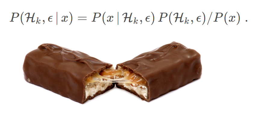
When we collect a datum such as \rm{DE} = \rm{VN}, we update our believes (probabilities) according to Bayes’ theorem:
P(\mathcal{H}_k, \epsilon\,|\,x) =P(x\,|\,\mathcal{H}_k, \epsilon)\,P(\mathcal{H}_k, \epsilon) / P(x)\;.where x is the datum and we can expand the probability to observe x into
P(x) = \sum_{k,i} P(x\,|\,\mathcal{H}_k, \epsilon_i)\,P(\mathcal{H}_k)\,P(\epsilon_i)\;.With a little bit of code, we can now explore how each datum changes our belief map, according to Bayes’ theorem above:
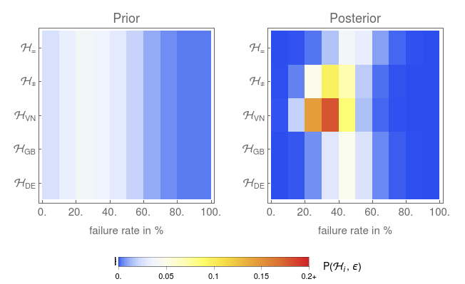
The most probable hypothesis is thus that the German and English Snickers bars are the same, but the Vietnamese Snickers bar is different (\mathcal{H}_{\rm{VN}}), and that our failure rate \epsilon is 30% to 40%.
The conclusion changes, however, when only mine or Nellissa’s measurements are taken into account. Here is a little video, where I explore the data with a little app I wrote.
Much more insight can be gained from the belief maps shown in the video above, but I leave this to you, dear reader, to think about the results. I, for my part, have had enough Snickers bars for a lifetime.