Semantic Map Embeddings – Part I
I originally published this on the Rasa blog.
How do you convey the “meaning” of a word to a computer? Nowadays, the default answer to this question is “use a word embedding”. A typical word embedding, such as GloVe or Word2Vec, represents a given word as a real vector of a few hundred dimensions. But vectors are not the only form of representation. Here we explore semantic map embeddings as an alternative that has some interesting properties. Semantic map embeddings are easy to visualize, allow you to semantically compare single words with entire documents, and they are sparse and therefore might yield some performance boost.
Semantic map embeddings are inspired by Francisco Webber’s fascinating work on semantic folding. Our approach is a bit different, but as with Webber’s embeddings, our semantic map embeddings are sparse binary matrices with some interesting properties. In this post, we’ll explore those interesting properties. Then, in Part II of this series, we’ll see how they are made.
Semantic Map Embeddings of Particular Words
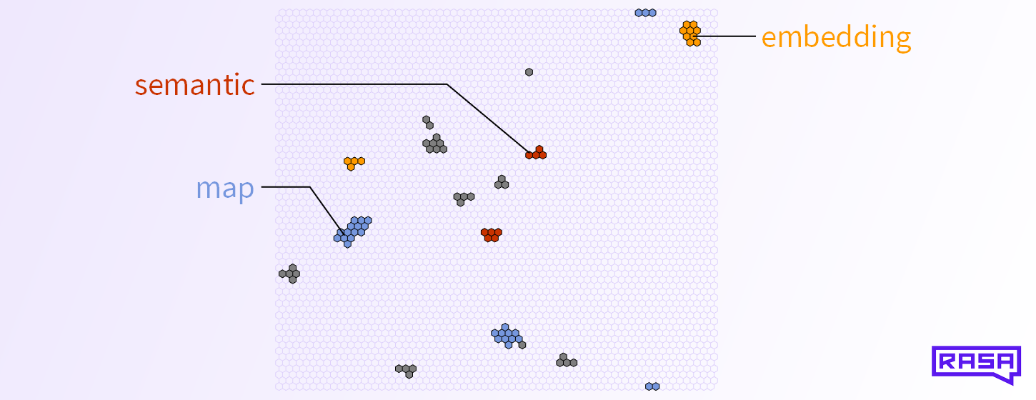
A semantic map embedding of a word is an M ⨉ N sparse binary matrix. We can think of it as a black-and-white image. Each pixel in that image corresponds to a class of contexts in which the word could appear. If the pixel value is 1 (“active”), then the word is common in its associated contexts, and if it is 0 (“inactive”), it is not. Importantly, neighboring pixels correspond to similar context classes! That is, the context of the pixel at position (3,3) is similar to the context of the pixel at (3,4).
Let’s look at a concrete example and choose M = N = 64. A semantic map embedding of the word “family” might look like this:

You may wonder why our image is made up of hexagons instead of squares. This is because we trained our semantic map in a way that each pixel has 6 neighbours instead of 4 or 8. We will describe in Part II how that training works.
Notice that the semantic map embedding of the word “family” is not a random distribution of active pixels. Instead, the active pixels cluster together in certain places. Each cluster of active pixels is also a cluster of similar context classes in which the word “family” appears. Larger clusters contain more context classes and might correspond to a whole topic.
We can see this if we compare the semantic map embedding of “family” with that of the word “children”:

The middle image shows the active pixels that both embeddings share. We can do this with a few other words and figure out what the different clusters stand for:

So each cell in the semantic map corresponds to a class of contexts, and neighbouring pixels stand for contexts that are similar. When a word’s particular meaning ranges across multiple very similar contexts, then you find clusters of active pixels on the map.
Semantic Similarity and the Overlap Score
In the previous section we have already seen that we can count the number of active pixels that two word embeddings share to compute a similarity score. How good is that score?
A simple thing we can try first is to pick a word and then find all the words in the vocabulary that have the most overlap with it. For example:


The size of the words in the word clouds corresponds to their overlap score with the target word in the middle (which is biggest because it has 100% overlap with itself). The higher the score, the larger the word. Looks pretty good!
We can attempt a more rigorous analysis and use the BLESS dataset, which is a list of word pairs and relation labels. For example, one element of the list is (“alligator”, “green”, attribute), i.e. “green” is a typical attribute of “alligator”. The different relations are:
| Relation | Description | Example with “alligator” |
| Typical attribute | green | |
| Typical related event | swim | |
| Meronym | “part of” relation | leg |
| Hypernym | “is a” relation | creature |
| Co-hyponym | Both terms have a common generalization | frog |
| Unrelated | electronic |
We compute the overlap between all the word pairs in the BLESS dataset. Ideally, all related words get a high score (maximum is 1) and all unrelated words (in the “Unrelated” category) get a low score (close to 0). Note, that a high score is only possible if the two words almost always appear together in any text. Thus, scores will mostly be below 0.5.
Here is how our 128×128 English Wikipedia embedding performs on the BLESS dataset:

This shows that our embedding captures all kinds of relations between words – especially co-hyponym relations – and less often associates supposedly unrelated words. This works because the matrices are sparse: the probability that you find a random overlap between two sparse binary matrices drops rapidly as you make the matrices bigger.
Still, many supposedly unrelated words do show high overlap scores. This seems to be not so great, except that many of the word pairs with the highest score in the Unrelated category are arguably quite related:
| Term 1 | Term 2 | Overlap Score (%) | Note |
| saxophone | lead | 56.1 | |
| guitar | arrangement | 49.4 | |
| trumpet | additional | 48.6 | |
| saxophone | vibes | 46.0 | |
| violin | op | 45.4 | “op” often stands for “opus” |
| robin | curling | 33.8 | “Robin Welsh” is a famous curling player |
| guitar | adam | 32.9 | “Adam Jones” is a famous guitar player |
| dress | uniform | 25.3 | |
| phone | server | 25.0 | |
| clarinet | mark | 22.6 | |
| cabbage | barbecue | 22.3 | |
| cello | taylor | 22.0 | |
| butterfly | found | 21.6 | |
| saw | first | 21.0 | |
| table | qualification | 19.2 | table tennis qualification |
| oven | liquid | 18.9 | see “polymer clay” |
| vulture | red | 18.6 | |
| ambulance | guard | 18.3 | |
| chair | commission | 17.4 | |
| musket | calibre | 17.1 |
Merging: How to Embed Sentences and Documents
We have introduced semantic map embeddings as sparse binary matrices that we assign to each word in a fixed vocabulary. We can interpret the pixels in these matrices and compare words to each other via the overlap score. But can we go beyond individual words and also embed sentences or entire documents?
Indeed we can! Semantic map embeddings offer a natural operation to “combine and compress” word embeddings such that you can create sparse binary matrices for any length of text. We call this the (symmetric) merge operation.
The merge operation does not take the order of the words into account. In that sense it is similar to taking the mean of the word vectors generated by Word2Vec embeddings. But in contrast to those traditional embeddings, our merge operation preserves the most “relevant” meanings of each word.
Let’s go through our derivation of the merge operation step by step. Our goal is to define a function MERGE that takes a list of sparse binary matrices as input and gives a sparse binary matrix as output. If the inputs are semantic map embeddings, then the output should somehow represent the shared meaning of all the inputs.
A naive way to combine the semantic map embeddings of words could be a pixel-wise OR operation. This does create a new binary matrix from any number of sparse binary matrices.

However, the combined matrix would be slightly more dense than the individual semantic map embedding matrices. If we were to combine a whole text corpus, most of the pixels would be active, and thus the OR-combined matrix would barely contain any information.

The next idea is then to add all the sparse binary matrices of the input words. As a result, we would get an integer matrix, and we could throw away all but the top, say, 2% of all active pixels, as those represent the context classes that are most shared by all the words in the text!

Now only one problem remains: if you want to merge just two words, then the top 2% are hard to determine, because all pixels will have values of either 0, 1, or 2. To remedy this final issue, we give extra weight to those pixels that have neighbours (more neighbours, more weight). We call the matrices with the weighted pixel values boosted embeddings. By doing this boosting, we not only get a more fine-grained weighting between the combined pixels, but we also emphasize those pixels of each word that carry the most likely meanings!

In summary, our merge operation takes the sum of all the boosted semantic map embeddings of the words of a text, then sets the lowest 98% (this number is arbitrary, but should be high) of all pixels to zero and the remaining 2% to 1. The resulting sparse binary matrix is a compressed representation of the meaning of the input text. For example, here is a semantic map embedding of Alice in Wonderland (the whole book):

We can now directly compare this semantic map embedding of the book with that of any word in the vocabulary. Here is a cloud with the words that most overlap with Alice in Wonderland:

This doesn’t look too bad, given that our embedding was trained on Wikipedia, which is arguably quite a different text corpus than Alice in Wonderland. What if we merge the text contents of the Wikipedia article about airplanes?


This word cloud also makes sense, though it seems to focus more on what airplanes are made of, or on technical things like “supersonic” or “compressed”. It doesn’t contain “flying”, but only “flew”. We think that this is an artifact of what Wikipedia articles are about. It’s an encyclopedia, not a novel. Also note that the word “components” does not appear anywhere in the article about airplanes, yet it is strongly associated with them.
Conclusion
That’s it for the interesting properties of this embedding. You can try our pre-trained semantic maps yourself, using our SemanticMapFeaturizer on the rasa-nlu-examples repo.
But how do we create these embeddings? In Part II we explore our unsupervised training procedure and compare our embeddings to BERT and Count-Vector featurizers.